Director: W. Jeffrey Hughes
Boston University
We all know weather, the daily changes in the atmosphere around us. Just as the dynamics of the atmosphere have important consequences, the mostly unseen dynamics of the Earth’s space environment are also important to us on the ground. Satellites can be destroyed by enhanced radiation or set tumbling by changes in the local magnetic field, communications and power distribution grids can be disrupted. As more of our technological base becomes dependent on space-based assets, the development of accurate forecast models for “Space Weather” becomes more and more important.
The National Science Foundation has recently funded a Science and Technology Center at Boston University, The Center for Integrated Space Weather Modeling (CISM), to address this need. The Center’s charter is to develop a model for space weather effects that runs from the surface of the Sun to the Earth’s atmosphere. Just as most weather prediction is no longer done by the seat of the pants but depends on detailed computer models, the task of the Center will be heavily dependent on numerical simulations of the development of space weather from where it starts on the Sun to where it finishes at the Earth. In this effort, CISM will be partnering with the Scientific Computing and Visualization group and the Center for Computational Science at Boston University.
The Space Weather Chain
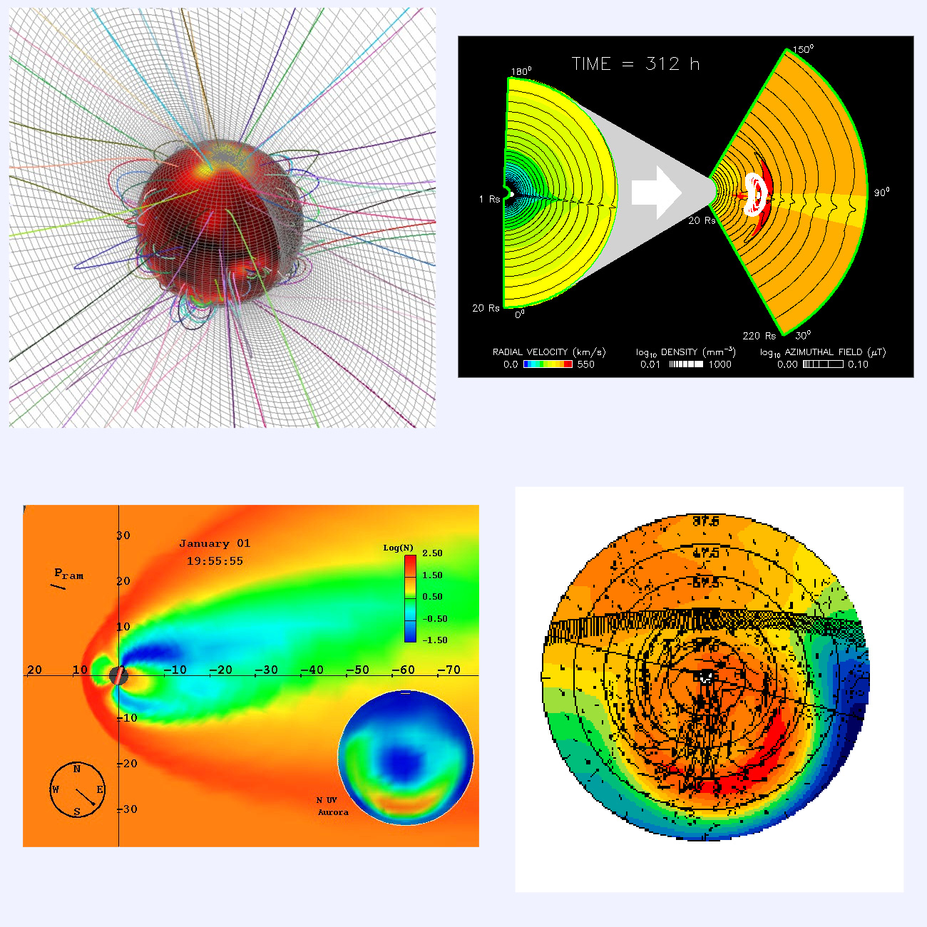
Figure 1 shows some of the simulations in this chain. We start at the Sun (upper left) where the dynamics of the coronal gas is calculated. Dynamics in this region and lower in the solar atmosphere can cause the eruption of large clouds of gas and magnetic field called coronal mass ejections (CME’s). These then propagate out through interplanetary space (upper right) increasing the speed and often the density of the gas flowing out from the Sun (the solar wind). The oval white area is a CME headed toward the Earth. This panel also illustrates some of the difficulties introduced by the volume of space that must be treated. The part of the corona seen in the upper left is a small inner part of the coronal calculation. The whole coronal calculation fits into a small region of the interplanetary model. The Earth literally cannot be seen on the scale of interplanetary space. The Earth is shielded from the direct influence of the solar wind and CME’s by its magnetic field, which holds off the solar wind flow, diverting it around the earth’s magnetosphere (lower left). However, the interaction of the solar wind with the magnetosphere creates a giant electrical generator that can cause electrical power equal to the entire electric generation capacity of North America to flow into the ionosphere at the polar caps (lower right). The lower right panel shows a picture of the ionosphere as seen from above the North pole. The color gives the total number of electrons in the ionosphere (red more, blue less). The orange band to the top is from the action of the solar ultraviolet flux, but the enhanced electron content toward the bottom (night-side) is from the electrical interaction with the magnetosphere.
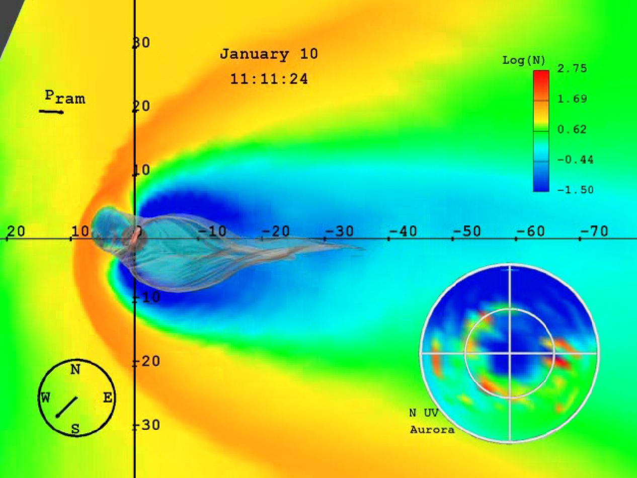
Magnetospheric Modeling
The second figure (above) expands on the magnetospheric panel above. The Earth sits at the intersection of the axes; the Sun is off to the left. The moon would sit at a distance near the -60 mark on the axis. The color code shows the logarithm of the density of the gas near the Earth. The solar wind is supersonic relative to the Earth and so the diversion of the solar wind flow creates a bow shock on the Sun side. On the opposite side there is a shadow region where the density is lowered and the magnetic field from the Earth is stretched out, the tail region. The gray translucent surface shows the boundary of the region where the Earth’s magnetic field totally dominates: compressed on the Sun side and stretched out on the tail side. This is a more or less normal magnetospheric situation, but it already hints at the complexity of the dynamics being modeled.
field and flows.
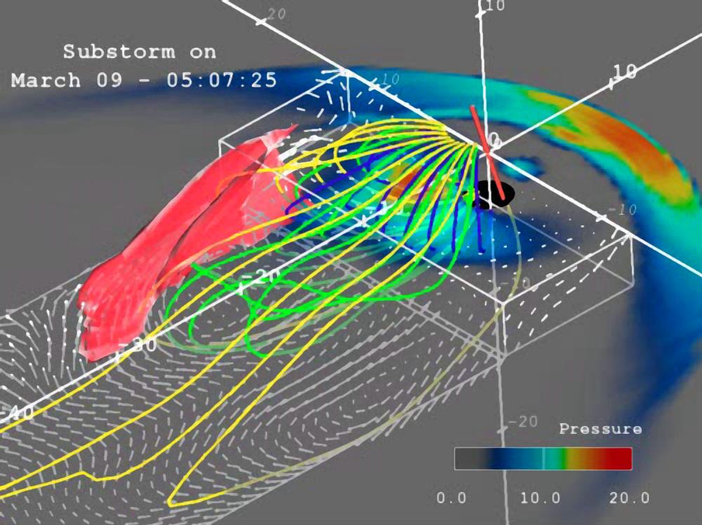
Figure 3 shows more of these dynamics. This panel shows a simulation of a period when there is an abrupt unloading of energy in the magnetosphere to the ionosphere, a substorm. An analogy to terrestrial weather might be a thunderstorm. Figure 3 looks from behind and above the Earth. The colored lines are magnetic field lines in the tail. Note how distorted they are relative to the natural dipole field that would exist without the solar wind interaction. The gray arrows in the plain show the direction and speed of fluid flow. Note the large scale eddies. The red surface shows a region of high-speed flow, generally toward the Earth. The color code case shows the pressure in the simulation.
The key point illustrated by the previous figure is the indication of the complexity that a simple physical model, ideal MHD, can produce. Other types of physics need to be considered for a complete picture of the Sun-solar wind-magnetosphere-ionosphere system. This leads to further complexity and to the computational issues of coupling different types of descriptions together. Putting it all together in a comprehensive model is the task of CISM.
The field of Space Weather prediction is at much the same point that terrestrial weather forecast was in the 1960’s, when the first computer models were being implemented. With the activity of CISM and its partners, SCV and CCS, Boston University is positioned to take a leading role in the development of realistic and worthwhile forecasting of the Earth’s space environment.