Forecasting Daily Demand for Hotel Occupancy Levels: An Empirical Application

By Apostolos Ampountolas, Ph.D., CQF, Assistant Professor of Finance and Revenue Management, Boston University – School of Hospitality Administration
Introduction
Over the past several years, the rapid development of information technology has been instrumental in the growth of demand in the hospitality sector. The new marketplace is becoming more competitive, which causes pricing pressure on the traditional service industries as the market supply increases. With this increase in prominent destination supply, and the number of new accommodation listings beyond the traditional purchasing options (e.g., sharing accommodation), new challenges on overnight demand related to forecasting and optimizing revenue have been created. Therefore, overnight forecasting is a key challenge for revenue managers because of the uncertainty associated between demand and supply. In the hotel industry, demand forecasting is challenging due to numerous anomalous days related to many annual holidays, various events, promotions, and environmental features that emerged. These new business models resulted in dramatic changes to the sales processes. Consequently, forecasting demand as an essential function for the hospitality industry stakeholders has developed new interesting forecasting models. To this point, although accurate forecasting is a critical component that affects revenue maximization, it estimated that a 20% reduction of forecast error translates into a 1% incremental revenue increase in a study for the airline industry by Pölt (1998). When deciding on a specific model, the model selection within forecasting is significant in itself.
Overnight demand forecasting
This study focuses on forecasting overnight demand by studying approaches to predict daily demand. Recent literature, see Pan and Yang (2017); Schwartz et al. (2016); and Pereira (2016), has looked at various techniques to examine the accuracy of hotel occupancy forecasts. Historically, each recommended method demonstrates drawbacks (van Ryzin, 2005) since many estimates use historical patterns to predict future estimation, while the market challenges the criteria for choosing forecasting methods. This leads to strong irregularity, along with seasonal patterns. The overnight demand exhibits variant arrival behavior that may contain outliers due to factors, such as promotions, holidays, and citywide events. In this context, the different types of datasets often incorporate daily, intra-week, weekly, monthly, and even intra-year irregular behavior that provides curves with a trend and seasonality. Therefore, daily demand structures are influenced by the strong effects of outliers, which adjusting and transforming to simplify the pattern can often lead to a more accurate forecast.
The models employed in most of the existing hospitality and tourism literature for the demand modeling and forecasting purposes include the vector autoregressive models (VAR and VECM) or Bayesian technique (BVAR), autoregressive moving average (ARIMA), analytical hierarchy process (AHP) exponential smoothing (ETS), time-varying parameter models (TVP), TBATS, choice modeling, and recently, more advanced machine learning (ML) models (see, Crouch, 1994; Law, 2004; Schwartz and Cohen, 2004; Wong et al., 2006; Haensel and Koole, 2011; Song et al., 2013; Pereira, 2016; Ampountolas, 2018; Ampountolas and Legg, 2021). Genuinely, in modeling, seasonality is usually examined by the seasonal autoregressive integrated moving average (SARIMA) model. Hotel daily demand exhibits several seasonal effects, such as weekly, intra-week, and weekend, with a period of seven days, in addition to the low, medium, and high-seasonal patterns with an annual seasonal pattern. Due to the nature of complexity, while employing high-frequency daily data, there is limited applied implementation on the hotel demand topic. Likewise, hotel demand exhibits high trends and seasonal patterns influenced by external factors, whereby traditional hotel revenue management forecasting is no longer entirely applicable. Consumer behavior and market observations justifying those daily forecasting procedures should be adjusted to trends and demand variations, incorporating data that strongly affect demand.
Evaluation of forecasting methods
Nowadays, different types of methods, from using legacy techniques to econometric models, are frequently employed to perform demand forecasting. Traditional quantitative forecasting methods include the time series as a set of observations generated sequentially in time and can be described by its stationarity (mean, variance, and autocorrelation function) (Hyndman and Athanasopoulos, 2018). Forecasts made at t time are needed at some future time t + l, that is, at lead time l, which vary with each problem and properties with an objective to obtain a probability accuracy as small as possible based upon the actual and forecasted values. Incorporating science to develop daily forecasting by including additional variables such as events and promotions, group business, and customer segmentation, revenue managers could produce optimized forecasting to improve accuracy and reduce uncertainties while optimizing their financial expectations and business performance.
In particular, several methods have been proposed in the hotel forecasting literature. Simple time-series models such as moving average, exponential smoothing, regression, and more advanced models such as the Autoregressive Integrated Moving Average (ARIMA) model in various forms and Machine Learning (ML) models have been applied for forecasting and are well-proven to be efficient. These statistical models usually exercise historical databases; however, the final outcome is under the prerequisite that selects the appropriate parameters. In light of the advanced algorithm modeling, artificial neural networks (ANN), which represent an important class of non-linear models, have shown impressive results in developing forecasting models for other industries.
This study aims to measure how successful neural network models perform comparably to simple alternatives due to the considerable interest in advanced forecasting models. Therefore, we evaluate the performance of our model with alternative prediction approaches to forecasting the daily demand, including a naive seasonal method, a Holt-Winters (HW) triple exponential smoothing model, and the multilayer perceptron (MLP) model, a neural network model (ANN). We recall that demand levels typically exhibit multiple fluctuations daily due to the strong effects of the exogenous indicators. Besides, an analysis of specific metrics has been applied to measure forecast accuracy: the Mean Absolute error (MAE), the Root Mean Square Error (RMSE), and the Mean Absolute Percentage Error (MAPE). Specifically, we evaluate if the improvements achieved in the empirical results will indicate more robust predictions for the overnight demand as the revenue management team relies on accuracy improvements. Finally, we considered the ANN as the benchmark forecasting model; thus, we measure the accuracy along each model forecast using the Relative Mean Absolute Error (RelMAE) measure. At the same time, if the proposed model will confirm the literature, which implies the effectiveness of advanced forecasting models towards comparative statistical models. The RelMAE measure is based on relative errors and is scale-independent. To measure the performance of ANN forecasts, we denote the MAE of ANN as a denominator for all evaluations. Therefore, when RelMAE > 1, then Method 2 is more accurate; when RelMAE < 1, the opposite is true, while if RelMAE = 1, methods are equally accurate (Barrow and Kourentzes, 2018).
Dataset and results
The data set of this study contains daily demand observations for a major hotel in a US metropolitan city over the period of April 1, 2017 to March 31, 2019. We divided the dataset into two segments, one used for fitting the model and another for testing the out-of-sample performance. We used the test set data from January 2019 to March 2019 to test the performance’s various forecasting models. The forecast horizon that is used to observe the demand is from 1 to 28 days ahead forecast.
Figure 1 shows the daily demand for the entire data set overtime period. The results indicate a stable demand over time, but with a notable increase trend presented by the black line, the estimated regression line. The trend shows periodic behavior within a month and year cycle. The overall mean for the monthly occupancy was 68.34% (μ = 68.34%), and the variance is 1.29%. The period between March 2018 to November 2018 shows a significantly increasing trend compared to the same period last year with an average demand of 65%. This time is considered as a low season with limited demand in any customer segment. In addition, the mean daily in the day of the week is quite similar daily, and the ratio between the variance to mean is significantly greater than one (1) every day.
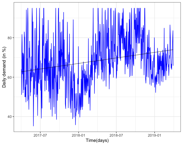
Figure 2 provides the average weekly plot of the data set on the day of the week. The weekly seasonality indicates intra-week demand patterns. The trend shows demand fluctuation similar to business hotels, where the demand performance is higher in the middle of the week (Tuesday, Wednesday) and adjusted slightly downward on Thursday, while demand on weekends shows a decrease. Besides, the intraday of the week demand shows a considerably similar pattern with data set demand over time. This pattern suggests that the daily demand is related to the type of hotel and market segment: retail, corporate customers.

An initial examination of the forecasting accuracy estimates disclosed that the differences in forecast accuracy within the models are moderate. On the other side, the gap between the first and the last horizon and the remaining forecast horizons (i horizons) generated substantial differences. It is obvious that accuracy measures generate conflicting results between the forecasting methods and the examined horizons. The model with the highest performance is highlighted in boldface across the horizons.
In this context, observations from the average RelMAE revealed that ANN outperformed the various models in four out of seven forecast horizons, while for remaining periods, the Holt-Winters and Seasonal Naive method performed best. The overall accuracy for the out-of-sample performance is demonstrated in Table 1. ANN performed better between horizons 3 and 14 than the other methods when we compare among other models according to MAE in Table 1. In the training of a neural network, we have tried different models with hidden layers and a number of hidden neurons. We assumed that the number of hidden layers could be between 1 to 3. Finally, we selected the best model based on the cross-validation error (12.593) with 3 layers and a model of 12 iterations (Figure 3a and b).

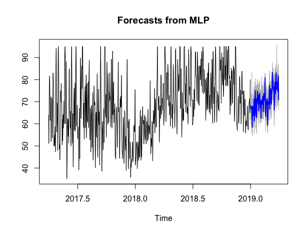
Figure 3: ANN model including exogenous features (a) ANN out-of-sample forecasting (b) model
Table 1: Average RMAE of forecasting methods
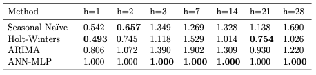
Figure 4 provides an additional comparison of each model’s results according to RMAE. For example, we observe that ANN is mostly outperforming all other models according to the RMAE measure.
Conclusions
In this study, using empirical results, we examine if the results will indicate more robust predictions for different models, including a feedforward neural network, the Multilayer Perceptrons (MLP), an Artificial Neural Networks (ANN) model with exogenous variables compared to the other statistical models. To measure the performance achieved by ANN, we have indicated ANN as the benchmark model for all evaluations. Observations from the average RelMAE revealed that ANN outperformed the various models in four out of seven forecast horizons. At the same time, for the remaining periods, the Holt-Winters and Seasonal Naive method perform best, verifying that seasonal, simple methods can outperform the more advanced ones (Taylor, 2010). The results are significant for revenue managers because it provides valuable insights into the exogenous outliers’ impact on establishing accurate daily demand forecasting.
Keywords: room nights demand prediction, deep learning, time series analysis, neural networks forecasting, hospitality, tourism
References