In scientific visualization the phenomenon under study is usually modeled by measurements at a discrete set of points in space. These may be thought of as representational samples of the the underlying mathematical function governing that phenomenon. There is often a mesh or “topology” associated with the points which enables interpolation of that implied function.
From a data point of view, we are working with a set of attributes (scalars, vectors, tensors, etc) attached to the set of points in space. The position of the data points may be given explicitly as (x,y,z) coordinates, or may by implicit (as in the case of a regular grid). In this section we will describe the most common forms which this takes.
The domains which we describe below may generally have arbitrary dimension. We will give illustrations of the 2-d version for clarity and simplicity, but we will describe the 3-d versions, since that is what occurs most commonly in scientific visualization applications.
Regular mesh. (Also referred to as a regular grid or uniform lattice.) This is probably the most commonly seen representation of the model domain because it is conceptually simple and clear, it corresponds naturally to array types provided by programming languages, and there is a large body of traditional mathematics organized around uniform samplings. All “grid lines” are parallel to coordinate axes, and the spacing between cells is uniform within each direction. There is an implicit “topology” of the underlying domain, by which we mean a set of “solid” cells which partition the domain, which can be used for interpolation.
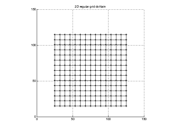
(Data in reg2Ddomain.txt.)
The location of any point in the grid can be determined from the index and the limits of the domain. For instance, in 3 dimensions:
x = xmin + ix*(xmax-xmin)    ix in [0,...,nx-1]
y = ymin + iy*(ymax-ymin)    iy in [0,...,ny-1]
z = zmin + iz*(zmax-zmin)    iz in [0,...,nz-1]
Note that the data is “attached to” these points, but the underlying scientific model which produced this data may be considering this data in one of two ways: the points may be at the corners of computational cells, in which case the boundaries of the domain lie at x=xmin, x=xmax, y=ymin, y=ymax, z=zmin, z=zmax; or the points may be at the centers of computational cells, in which case the boundaries of the computational domain are a half step width beyond the given mins and maxs.
Perimeter mesh. (Also referred to as a perimeter grid or rectilinear lattice.) This is similar to the regular mesh described above, except that the spacing in each dimension may be non-uniform.
In addition to the information given for the regular grid, we need lists of the coordinate positions in the x, y, and z directions.
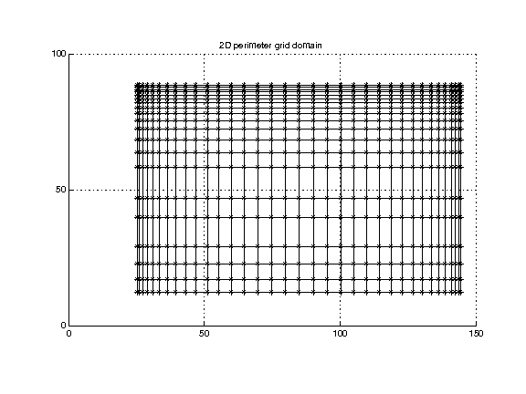
(Data in perim2Ddomain.txt.)
The location of any point in the grid can be determined from the index and the limits of the domain. For instance, in 3 dimensions:
Representation:
x = xgrid[ix]    where ix in [0,...,nx-1]
y = ygrid[iy]    where iy in [0,...,ny-1]
z = zgrid[iz]    where iz in [0,...,nz-1]
xgrid = (x_0, ..., x_{n-1})
ygrid = (y_0, ..., y_{n-1})
zgrid = (z_0, ..., z_{n-1})
Irregular mesh. (Also referred to as an irregular grid or curvilinear lattice.) Here the topology is the same as above (the cells are quadrilaterals in 2-d, cuboids in 3-d) but the points lie in arbitrary locations. The connectivity between points is implicitly given by the mesh structure (essentially by indexing), but the coordinates of each point need to be listed explicitly.
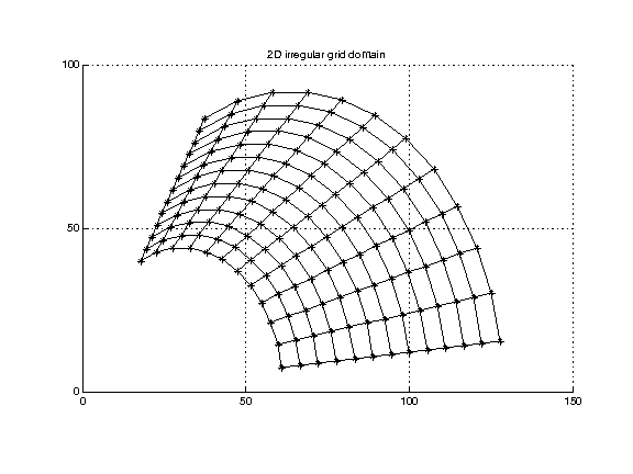
(Data in quad2Ddomain.txt.)
Representation:
x_0 y_0 z_0
x_1 y_1 z_1
...
x_{n-1} y_{n-1} z_{n-1}   n = nx*ny*nz
In any of the grid representations above, an important factor which varies with different packages and programming language is how the points are ordered in the grid, i.e., how the 1-d list of points in computer memory is mapped onto the multi-dimensional grid in space. Common terminologies talk about x (or y or z) “varying fastest, which means that adjacent data points in the list correspond to marching along the x (or y or z) dimension of the grid.
Triangulated domain. Here the cells are not cuboids but are triangles (tetrahedra).
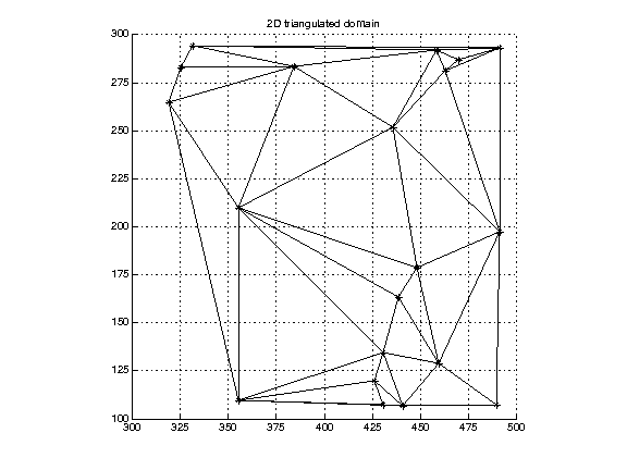
(Data in tri2Ddomain.txt.)
Representation:
x_0 y_0 z_0
x_1 y_1 z_1
...
x_{3*n-1} y_{3*n-1} z_{3*n-1}                 where n is the number of triangles
or an indexed version:
x_0 y_0 z_0
x_1 y_1 z_1
...
x_{n-1} y_{n-1} z_{n-1}
index_0_0 index0_1 index_0_2                  indices of vertices of 0
...
index_{nt-1}_0 index{nt-1}_1 index_{nt-1}_2   indices of vertices of nt-1
                                              where nt is the number of triangles
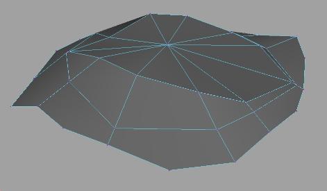
Polygonal domain. Here the cells may have different numbers of vertices, edges, etc, so the elements need to be specified explicitly. In 2-d listing the vertices in order is enough to specify a polygonal cell. In 3-d, specifying the vertices is enough if we know that cells are convex. If not, in general we need to give explicit information about edges and/or faces.
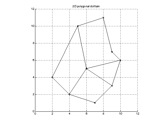
Representation in 2-d:
x_0 y_0
x_1 y_1
...
x_{n-1} y_{n-1}
index_0_0 ... index_0_{k_0}                indices of vertices of polygonal 0
...
index_{np-1}_0 ... index_{np-1}_{k_{np-1}} indices of vertices of polygon np-1
The analogy in 3-d (irregular 3-d cells partitioning space) is somewhat more complicated, and arises rarely in sci vis, so we will not give more details on the computer representation here.
Discrete points. We have no other information about their relation to each other. These may be randomly chosen sample points, or data from sensors at particular geographic locations, etc.
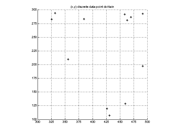
(Data in discrete2Ddomain.txt.)
Representation for each curve of “length” n:
x_0 y_0 z_0
x_1 y_1 z_1
...
x_{n-1} y_{n-1} z_{n-1}
Curves. These are piecewise linear (1-d) objects embedded in the plane, or space. 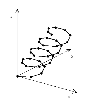
An individual curve may be represented as a list of explicit points or as a list of indices into a set of points, in an analogous manner to that for triangle meshes, above.
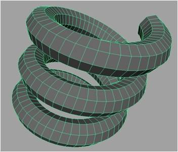
Surface. These are 2-d objects embedded in space. The geometry is generally represented in the same manner as that described above for polygonal meshes in the plane.
x_0 y_0 z_0
x_1 y_1 z_1
...
x_{n-1} y_{n-1} z_{n-1}
index_0_0 ... index_0_{k_0}                indices of vertices of polygonal 0
...
index_{np-1}_0 ... index_{np-1}_{k_{np-1}} indices of vertices of polygon np-1