MR Data Quality Control
- Quantitative QC: Automatic QC via XNAT
- What is the QC pipeline in XNAT?
- How do I run the QC pipeline in XNAT?
- How do I access the data?
- What do the produced reports look like?
- Qualitative QC: Looking at your data
Quantitative QC: Automatic QC via XNAT
What is the QC pipeline in XNAT?
The pipeline was created by Tim O’Keefe from Harvard. It consists of two pipelines, BOLDQC (https://boldqc.readthedocs.io/en/latest/) and ANATQC (https://anatqc.readthedocs.io/en/latest/). They both perform minimal processing on the data to pull out basic QC measures. ANATQC is build on top of dcm2niix, FreeSurfer, vNav, and MRIQC packages. BOLDQC is built on top of dcm2niix, FreeSurfer, and FSL.
How do I run the QC pipeline in XNAT?
The pipeline should be automatically run on all BOLD and MEMPRAGE (standard structural) scans. If you find one of your datasets that does not have it run, and is more than a day old, please contact Kyle via Research Computing Systems ticketing system: help@scc.bu.edu.
How do I access the data?
Since the data is run on an individual run basis, there will be data for each BOLD and ANAT that the pipeline was run on. You can view data for an individual run from the view link that gets added into the main view of your data:

The pipeline also adds flags to the Notes column. If there isn’t a flag there, then the pipeline didn’t pick it up as a valid run. If you think it missed a run that should have been processes, please contact Kyle via Research Computing Systems ticketing system: help@scc.bu.edu.
What does the ANATQC report look like?

QC Metrics
There are several metrics on the left. They are color coded if they are coming from Freesurfer or MRIQC.
These metrics can vary depending on the parameters of your structural scan. We are still building up data to get a better sense of the variability of these metrics for commonly used protocols at the center. For general guidelines, see here.
Images tab
The images are described below. To make them bigger in XNAT, you can click on an image.
- Top left: T1w, want to have the whole brain, no wrapping, uniform contrast.
- Top right: Freesurfer white matter and pial surface segmentations, want to generally be grabbing the brain, and following the gray matter ribbon.
- Botton left: Freesurfer subcortical and cortical segmentations, you want subcortical segmentations to look generally good, and cerebellum.
MRIQC tab

You can find more detailed information on the MRIQC report on their website
For a quick description:
- Background image: make sure there ins’t any ghosting or wrap around.
- The zoomed in Mosaic: make sure everything is clear, not too much banding.
- Artificial Intensities on the Background: looking for stripping or lots of background noise that might indicate RF noise.
- Spatial normalization of the anatomical image: this is a quick pass at alignment to template space. If it looks generally ok, you should feel more confident that your own transformation to common space will go smoothly.
MRIQC IQM tab

This table gives you all the QA metrics MRIQC creates. This can be used to create distributions across your participants to give you an idea of the distribution of your data to identify outliers.
Manual QC tab
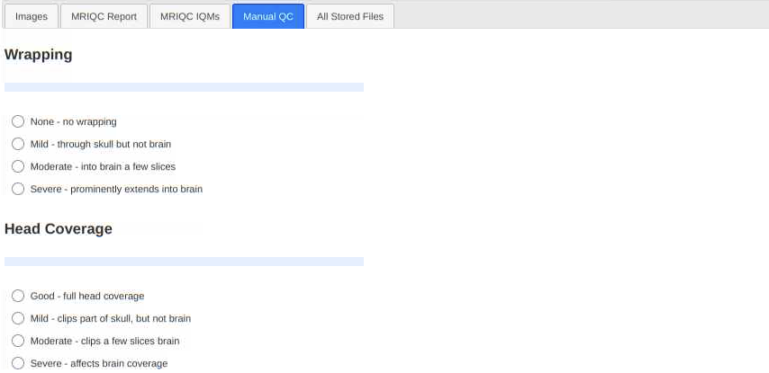
In this tab, you can record overall ratings of the data, which can later be read by other users or can be used to filter ‘usable’ data in the database. This is most useful for large datasets, or datasets multiple groups might access, such as in a public release. There are several criteria by which data can be classified. These mainly need to be assessed via qualitative inspection of your data. Then, there is a final overall QC assessment rating that can be set.
All Stored Files tab
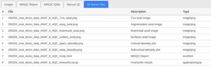
This tab lists all the stored files that are created. Generally, this is not data you would use, as you don’t have the ability to edit the pipeline. For instance, if the Freesurfer segmentation doesn’t go well, you can’t change the needed variables to correct it and rerun it. Therefore, you generally would only want to download the MRIQC report.
Important metrics from ANATQC
The metrics from ANATQC can vary by the protocol used to collect the data, such as how much acceleration is used. Therefore, the best way to determine what is ‘good’, is to create distributions of your own data and set outlier thresholds. For structural scanning, there is a smaller subset of protocols used in the center, so we hope to be able to calculate some averages for our data. For now, the Harvard folks have generally found that:
SNR total: less than 8 is concerning. For populations with more movement, less than 9.5 is a good threshold.
What does the BOLDQC report look like?

There are several metrics on the left. First are basic parameters for the run. Make sure the number of volumes is correct, and that the mask threshold is consistent with other participants and runs.
Second are the QC Metrics. For a more detailed description of what guidelines to use, see below.
Images tab:
- Top left: Voxel SNR map
- Formed by dividing the mean map (middle map) by the standard deviation (right map).
- Generally, it will take some practice in looking at these maps to tell what is ‘normal’, and this varies by coil. For the 64ch, these are generally brighter at the edges of the brain.
- Middle left: Slope Map
- Calculates changes over time, and therefore can be useful in highlighting movement. Areas of white or black have large movement.
- Middle Center: Mean slice intensity over time
- You want these lines to be fairly smooth
- Middle Right: Motion parameters
- From MCFLIRT (affine registration, FSL)
- You also want relatively small changes.
- Pay attention to the axis scale closely to assess the magnitude of movements, as it is scaled differently for each report.
- Bottom: Mask
- You want this to be generally uniform and covering the whole brain. If there are areas of drop out, this might suggest regions of low signal.
Automated QC tab:

This tab shows a few more measurements than the main summary page, in addition to everything on the summary page.
Manual QC tab:

In this tab, you can record overall ratings of the data, which can later be read by other users or can be used to filter ‘usable’ data in the database. There are several criteria by which data can be classified. These include motion, head coverage, signal homogeneity, ghosting, and RF noise/spiking. Motion can be assessed with the quantitative values that come out of BOLD QC, while the rest need to be assessed via qualitative inspection of your data. Then, there is a final overall QC assessment rating that can be set.
All Stored Files tab

This is where the files created are listed. You can click on any of these to download the files. Generally you do not want to be downloading the processed data as you do not have any control over what was run, no ability to fix errors, or necessarily hold the version of software used constant. The auto_report.txt file contains the statistics from BOLDQC that can be used to qualify data. This is useful to download the summarize across your participants to look for outliers.
The auto QC report contains the parameters in the parameters box on the left, in rather cryptic names:
- qc_sSNR = slice SNR
- qc_vSNR= voxel SNR
- mot_rel_xyz_mean = Mean Relative Motion
- mot_rel_xyz_max = Max Relative Motion
- mot_abs_xyz_mean = Mean Absolute Motion
- mot_abs_xyz_max = Max Absolute Motion
- mot_rel_xyz_1mm = Number of movements > 0.1mm
- mot_rel_xyz_5mm = Number of movements > 0.5mm
Important metrics from BOLDQC
The metrics from BOLDQC can vary by the protocol used to collect the data, such as how much acceleration is used or how big the voxels are. Therefore, the best way to determine what is ‘good’, is to create distributions of your own data and set outlier thresholds. As a starting place, the Harvard folks have created some guidelines after looking at lots of data.

- Slice SNR:
- SNR greater than 150 good, while less than 99 is bad (for Siemens 3T 12ch adult data).
- Max Abs Motion:
- Values less than 1.49 are good, while greater than 2mm is bad.
- Movements (>.5mm):
- Number of movements greater than 0.5mm should be less than 5 for good data, greater than 5 is bad. This is calculated as the root mean square of movement in 3D space.
There are many other variables listed that you might find useful, but for which hard guidelines haven’t been created for. For instance, voxel SNR (timecourse SNR calculated for each individual voxel) is more dominated by scanner noise than slice SNR and might be useful. So might be max or mean relative motion, which is movement relative to the previous volume as opposed to the first volume.
Qualitative QC: Looking at your data
How do I perform qualitative QC on my structural data?
Qualitative QC involves looking at your data. We recommend doing this via FSL. This does not mean you need to analyze your data in FSL, but the FSLeyes just has a nice interface to visualize the nifti files. After you finish the qualitative QC you can enter your findings into XNAT using the manual tab if you like. For a better description of the various artifacts, see the QC manual (pdf) that was created by Natasha Hansen and others at Harvard/MGH. It includes several things we don’t really see anymore with the newer coils and protocols, but still useful!
- Load FSL into your environment, it doesn’t matter which since we are just viewing data.
module load fsl - Load your structural scan.
fsleyes structural_name & - Scroll through all the slices in each view of the brain.
- Verify that that all of the brain is there (not clipped)
- Verify that if any part of the anatomy fell outside of the field of view and is wrapping around, that it doesn’t overlap with the brain.
- Look for artifacts in the ‘ringing’, ‘striping’, and ‘blurring’ category. These artifacts can sometimes be easier to see if you use Single View (Tools > Single) to enlarge the view of the axial plane.
- Look for radio frequency (RF) noise, which resembles TV static over the scan image, and spiking, which looks like rigid stripes over the brain and/or background.
- Look for susceptibility artifacts (a black area of signal loss surrounded by bright and dark ripples – such as in the mouth when participants have a permanent retainer).
- Turn on Lightbox View (Tools > Lightbox) and scroll down to slices that show the full walnut shape of the brain. Decrease the contrast by lowering the max brightness value while leaving the minimum brightness as the default value (0). Lower the max brightness to 1/3 the default value. Scroll through all the slices:
- Look for ghosting (a fainter displaced copy of the head, brain, or eyes).
- Pay attention to where the ghost image might overlap with the brain.
- Look for RF noise. With this contrast, a little RF noise (TV static) is normal, but you should check if there is more than usual. You should not see rigid stripes (spiking).
- Reset the brightness values to default. Then increase the contrast by raising the minimum brightness value while leaving the maximum brightness value at the default. Raise the minimum brightness to 1/3, then 1/2, then 2/3 of the maximum, each time scrolling through all the slices in each view of the brain.
- Look for the homogeneity of the signal intensity. This will depend partly on the scanner and coil, but in general the outer rim of the brain is brighter than the interior. The signal homogeneity pattern should be symmetrical, particularly left to right. In general, it should also be symmetrical front to back, but can depend on how the subject’s head was padded, particularly if they have a small head and are far away from the coil, as with children.
How do I perform qualitative QC on my BOLD data?
Qualitative QC involves looking at your data. We recommend doing this via FSL. This does not mean you need to analyze your data in FSL, but the FSLeyes just has a nice interface to visualize the nifti files. After you finish the qualitative QC you can enter your findings into XNAT using the manual tab if you like. For a better description of the various artifacts, see the QC manual (pdf) that was created by Natasha Hansen and others at Harvard/MGH. It includes several things we don’t really see anymore with the newer coils and protocols, but still useful!
- Load FSL into your environment, it doesn’t matter which since we are just viewing data.
module load fsl - Load your functional data. You will have to perform QC for each BOLD run. If you are using FSL, type:
fsleyes functional_name & - Check for head coverage, make sure all of the brain target area (the part you care about for your study) is covered and not clipped by the edge of the field of view.
- Remember to scroll through all the slices in the coronal plane to check if the bottom tips of the temporal lobes are cut off.
- Turn on Movie mode. This will automatically cycle you through the timepoints (volumes), so you will be more likely to spot issues that are timepoint-specific as you scroll through the slices. Continue to scroll through the slices, making sure that movie mode plays through a full cycle of volumes and starts over at zero (0) several times.
- Look for motion slice artifact (sudden horizontal light and dark stripes through the brain that may only be there for particular timepoint(s).
- Look for RF noise (like TV static) and spiking (sudden extreme static and/or stripes through the brain). Mild-moderate degrees of RF noise can be more easily seen when you decrease the contrast (see step 7 below).
- Turn on Lightbox View (Tools > Lightbox) and increase the view size to 200%.
- Scroll though all the slices in each view of the brain.
- Decrease the contrast by lowering the maximum brightness value to 1/3 the default while leaving the minimum value at the default (0). Scroll through the slices in each plane:
- Check for ghosting (a fainter displaced copy of the brain). There will always be some amount of ghosting, but check how visible it is and is if it overlaps the original brain image.
- Look for RF noise and spiking again.
- While leaving on Lightbox and Movie mode, reset the contrast to its default values. Then increase the contrast by raising the minimum brightness value while leaving the maximum at the default. Raise the minimum brightness to 1/3, then 1/2, then 2/3 of the maximum, each time scrolling through all the slices in each plane.
- Look for the homogeneity of the signal intensity. You will get to know what looks normal for your scanner and coil, but in general the outer rim of the grain is brighter than the interior. The signal homogeneity pattern should be symmetrical left to right. In general, it should also be symmetrical front to back, but this can vary depending on how people are padded, especially if they have a small head, as with children.