The Magic Hat: an adaptive solution for enhancing visually guided mobility of the visually impaired

(Grant No. CDA-9528079 Award date: August 2, 1995)

Principal Investigator: Lucia M. Vaina

Co-Investigator: Sundareswaran Venkarataman

Brain and Vision Research Laboratory
Biomedical Engineering, College of Engineering
Boston University

Report

(Note: For fast loading, please copy the folder containing this document to hard disk)In this document, we report the methods that have been developed in the Magic Hat project (NSF SGER grant CDA-9528079) for collision warning based on visual information.

Summary of the grant proposal

The goal of the project is to demonstrate the feasibility of a device capable of warning blind and low vision people about impending danger (collision), by processing visual motion information. The primary consideration was to develop a collision warning method that is fast, and can be demonstrated using existing technology in as close to real-time as possible.

Visual motion information is obtained by processing sequence of video images from an off-the-shelf camcorder. Our implementation of collision detection has the following set-up:

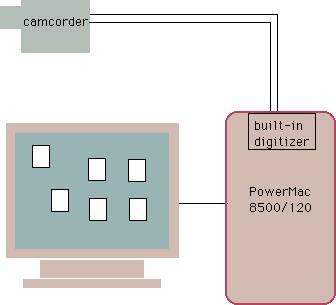
Magic hat schematic diagram — Figure 1. Schematic of the collision detection demo set-up

The NTSC signal from the camcorder is digitized by the built-in digitizer. The digitizer action is controlled from Collision Demo, a modified version of the public-domain program NIH Image. Collision Demo works at about 3 frame s per second on the PowerMac 8500/120, and provides warning about impending collisions. The general outline of the collision warning method is as follows:

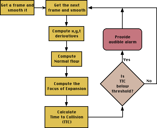
Collision detection flow-chart — Figure 2. Flow chart of the collision warning method

We explain each of the steps in detail below:

Computation of derivatives
The x,y, and t derivatives are computed from two subsequent frames in the following way. First, the two frames are smoothed (within the processing loop, only the current frame is smoothed, the earlier frame has been smoothed in the previous iteration). Th e smoothed first image is convolved with x and y derivative kernels shown below:

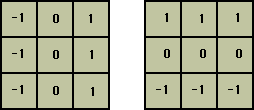
X and Y derivative kernels — Figure 3. x and y derivative kernels

Results of applying this kernel on an image are shown in the figure below. The image, its x-derivative and y-derivative are shown, respectively from left to right.

Derivative images — Figure 4. An image, its x-derivative, and y-derivative

The temporal derivative is computed as the pixel-wise difference between the two smoothed frames.

Flow computation
Normal flow is computed at locations where the local spatial gradient magnitude is above a threshold value. The gradient method based on the optic flow constraint equation shown below is used to calculate the normal flow:

Near-flat intensity distribution and noisy spots give rise to large normal flow magnitude, and rounding approximations give rise to small flow measurements where none exitst. Thus, normal flow measurements with very low or large magnitude are ignored.

If the size of the moving region is larger than a threshold, the 3D motion is considered to be self-motion; otherwise, the moving object is isolated and all further processing is restricted to the moving object (the moving object is enclosed by a white re ctangle in the display window).

FOE Computation

The focus of expansion (FOE) is computed based on the principle that flow vectors are oriented in specific directions relative to the FOE. The horizontal component h_Lof an optic flow vector Lto the left of the FOE points leftward. For an optic flow vector R to the right of the FOE, the horizontal component h_R points rightward, as shown in the figure on the left. By a c ounting method, we can determine the location about which a majority of horizontal components diverge. We have extended this principle to the field of normal flow vectors. Thus, we can find the FOE from a normal flow vector field, providing that the inten sity gradient (edge) distribution in the image is uniform (i.e., the probability that a certain orientation is seen in an image location is the same as for any other orientation). The proof for this method is given in the Appendix.

Computation of Time to Collision (TTC)
The time to collision (TTC) can be computed from the parameters of the first-order approximation to the optic flow field. The first-order (affine) approximation is given by

The parameters a₂ and a₆ encode the divergence of the flow. It can be shown that for surfaces that give rise to a flow that is nearly affine, the TTC is giv en by the expression TTC expression

. The parameters a₂ and a₆ can be computed from the normal flow over a 2-D regio n. However, to speed up the computation, we consider only the horizontal line and the vertical line passing through the FOE. The following figure illustrates the simplification achieved by this choice:

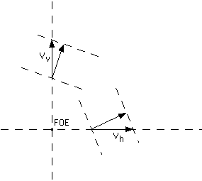Arbitrary local edge directions have been chosen to show the normal flow of two optic flow vectors-one along the vertical line and the other along the horizontal line passing through the FOE. Note that these optic flow vectors must lie along these li nes because of the structure of translational flow fields. It can be easily shown that the magnitude of the horizontal optic flow vector is and that of the vertical opti c flow vector is , where E is the spatio-temporal intensity function. These derivatives have been computed earlier. From several measu rements along the horizontal and vertical lines, we can calculate the desired affine parameters as follows:

,where x_h and y_v are transformed coordinates with the FOE as the origin. The TTC can now be computed. If the TTC is below a pre-set value, an audible alarm is sounded, and the look-up table of the output image is inverted (i.e., a “negative” image is displayed).

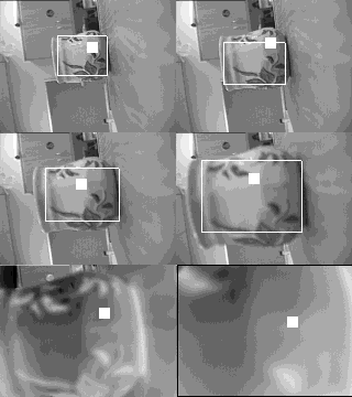
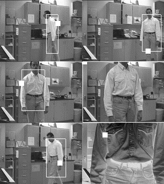
Shown below are results from some image sequences. If object motion is sensed, a white rectangle is drawn around the object. The FOE is shown as a small white square. No temporal integration is performed (all results are based on 2-frame processing). The first two sequences (the pretzel box sequence and the coffee cup sequence were shot off-line and then processed; the lab walk sequence was processed on-line). All the imag e sequences were a fourth of normal NTSC size: 120 X 160 pixels. The speed of the animation is not related to the speed of processing (various factors come in to play, including the speed of the machine on which the browser is running). We estimated empir ically that our implementation in NIH Image v1.60 running on a PowerMac 8500/120/32M runs at 3 frames/sec. We believe that a hardware implementation will run in real-time.

Figure 5. Sample result sequences demostrating collision warning

Discussion

Advantages of this method
There are several advantages to our approach. We list them below:

Performance can be scaled up to real-time levels by hardware implementation. The simple computational steps can be easily implemented in currently available hardware.
No camera calibration information is required. For the TTC computation, inter-pixel distance is required, but this may be specified in arbitrary units (e.g, pixel count, as in our implementation) because the “collision sensitiv ity” can be adjusted to compensate for the unknown scale factor.
The implementation can be done in most off-the-shelf framegrabbers and cameras. No special equipment is needed.
Due to the simplicity and reliability of the computations, the approach can be extended for low-light situations or infra-red image sequences.
The approach can be easily modified for tracking and motion encoding applications.

Edge Distribution

Even if the FOE computation seemed to work well, we wanted to ascertain that the edge distribution in the images was as assumed (uniform: see the appendix). We modified the FOE computation program to calculate the edge distributio n in indoor images (sequences). The advantage of modifying the FOE program (instead of writing a new one) was that the statistics considered only edges of the same type (satisfying the same gradient and velocity thresholds) as in the FOE computation. Res ults from a typical indoor scene are shown below: first a sample image from the sequence, second the distribution of the edge orientations (0 degrees corresponds to horizontal, 90 degrees is vertical).

Figure 6. A typical indoor image, and edge distribution of a sequence containing this image

Contrary to our assumption (but consistent with empirical observations in the literature on statistics of indoor images), we found a skewed distribution, with peaks corresponding to the horizontal and vertical edges. However, an analysis of the effect of this skewed distribution suggests that a preponderance of vertical and horizontal edges will not affect-and in fact enhance-the performance of our FOE detection algorithm, provided that the 3-D horizontal and vertical edges are projected as horizontal and vertical edges on the image plane (not necessarily in that order-for e.g., a vertical edge could project as a horizontal edge on the image by rotating the camera by 90 degrees). This is due to the fact that we use the horizontal and vertical axes as our reference frames to project the components of the normal flow (see the explanation for vertical edges in the appendix). The preceding observations do not imply, however, that the method will fail when the distribution of edges is skewed in an unfavorable fashion. In order to perform a complete analysis of failure, we should consider not only the edge distribution, but also the motion direction distribution. Since this joint distribution is not well-studie d, we will not conduct the extended analysis. We conclude by noting that in all real, indoor sequences that we processed, the collision warning computation was successful.

Appendix A

Here we prove a theorem that allows us to use normal flow to determine the focus of expansion, providing (a) the 3D motion is translational, and (b) there is a uniform distribution of edge orientations.
Theorem:With high probability (greater than 0.5), the signs of the components of a normal flow vector agree with the signs of the components of the corresponding optic flow vector, providing the local intensity gradient direction is distributed uniformly.

Proof:
Let the local gradient subtend an angle a, and the optic flow vector subtend an angle q, with the x axis. Without loss of generality, we can assume that both a and q are in the range 0 to p/2 (p*d is the circumference of a circle with diameter d). The loc al gradient is along [cos(a), sin(a)] and the optic flow vector is along [cos(q), sin(q)]. The normal flow vector is in the direction cos (q-a)[cos(a), sin(a)].

For the x component of this (normal) vector to have the same sign as the x component of the optic flow vector,

cos (q-a) cos (a) cos(q) > 0.

We consider two possibilities:
1. cos (q-a) > 0 and cos (a) cos (q) > 0, or
2. cos(q-a) < 0 and cos (a) cos (q) < 0.

The first situation occurs if |q-a| < p/2, and if a and q are in the same vertical set of quadrants (first and fourth, or second and third). For a given q , a has a range of p-q in which an agreement of signs results. For the second situation, | 2 p + q – a | < p/2, and a and q must be in in the same horizontal set of quadrants (first and second, or third and fourth). This corresponds to a range of p-q for a. Since the total possible range for a is 0 to 2 p, assuming a uniform distribution for a,the prob ability that the signs of the x components agree is ( p – q ) / p.

In passing, we note that for a =0, p (vertical edges), the signs of the x components always agree!

Using a similar argument, it can be easily shown that the probability that the y components agree is (p/2+q )/p.