The isosurface for a given value d is the set of all points in the domain for which the function has the value d. Under a fairly common set of conditions this set is a surface or set of surfaces.
In 2D this concept reduces to an isocurve or isoline. If the reader is familiar with topographical maps, the isocurve is the same thing as a contour line. The isosurface is the 3-d analog of an isocurve.
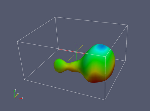
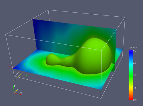
Here is an example of an isosurface, for the same data set we have been looking at, for a particular value.
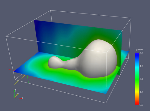
Combining it with the horizontal and vertical slices we used previously gives more information in one image.
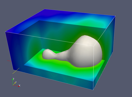
We can do the same thing using the brick clipping technique.
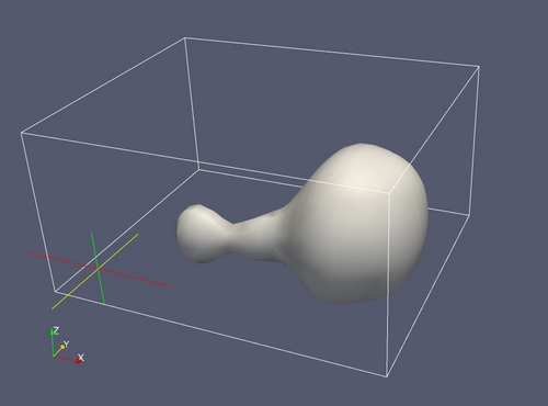
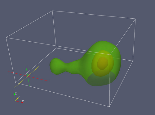
If we render the isosurface as a translucent material, in a sense we have access to all the information.
![]()
It is sometimes useful and intuitive to color the isosurface using the same pseudocolor map as used for the rest of the visualizations. This becomes even more useful/important when presenting isosurfaces for multiple values, whether in the same graphic or in separate ones.
Transparency can be used in combination with coloring of the isosurface.
![]()
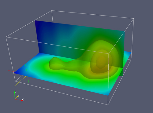
Trying to see multiple solid isosurfaces in one image tends not to work well, because they usually form a set of nested surfaces. Combining transparency and color when rendering multiple isosurfaces solves this problem.
This can be combined with the slice planes.
The isosurface gives information about one parameter. We may be interested in knowing the behavior of another property on that surface. We can do this by using the second parameter to color the isosurface (mush as we colored slice planes).